ISMRM Sunrise Practical Session

This document contains the second set of practical exercises for the ISMRM course on parallel imaging.

Excercise Data
Noise Pre-Whitening
SNR Scaled Reconstruction
Pseudo Replica Method
Iterative Non-Cartesian SENSE
Additional Demos

Excercise Data

All the data used in this set of exercises can be found in the file hansen_exercises.mat. We will start by clearing the workspace and loading the data

close all; clear all;
load hansen_exercises.mat
whos

  Name                  Size                 Bytes  Class     Attributes

  data                256x256x8            8388608  double    complex   
  data_spiral       18176x8                2326528  double    complex   
  k_spiral          18176x2                 290816  double              
  noise_color         256x256x8            8388608  double    complex   
  noise_spiral      18176x8                2326528  double    complex   
  reg_img             256x256               524288  double              
  smaps               256x256x8            8388608  double    complex   
  sp                  256x256               524288  double              
  w_spiral          18176x1                 145408  double

Noise Pre-Whitening

The purpose of this exercise is to see the effects of noise
pre-whitening. We will use a SENSE reconstruction as an example

$\tilde{\mathbf{x}} = \arg \min_{\mathbf{x}} \left\{ \left\| \mathbf{E}\mathbf{x}-\mathbf{m} \right\|_2 \right\}$

where $\mathbf{x}$ is the reconstructed image, $\mathbf{E}$ is the encoding (sensitivity matrix) and $\mathbf{s}$ is the measured data.

Let's start with a naive SENSE reconstruction

smask = (sp == 1 | sp == 3);
ncoils = size(smaps,3);
nelements = numel(smaps)/ncoils;

acc_factor = (numel(sp)/sum(smask(:)));
unmix = ismrm_calculate_sense_unmixing(acc_factor,smaps);

alias_img = ismrm_transform_kspace_to_image(data .* repmat(smask,[1 1 ncoils]),[1,2]);

Let's look at the aliased images:

ismrm_imshow(abs(alias_img),[],[2 4]);

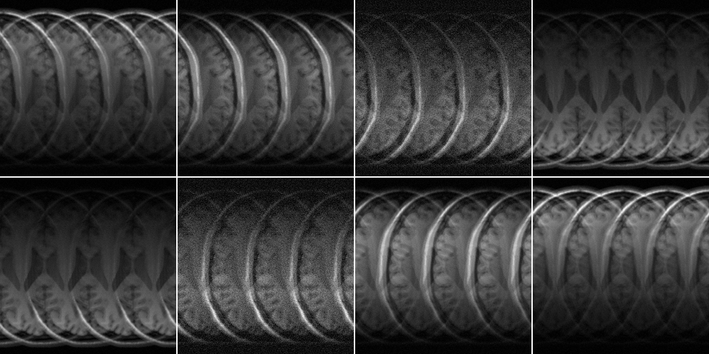
It is evident already from this view that a couple of channels have a different noise level (channels 3 and 6).

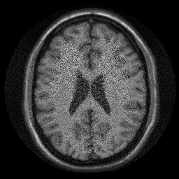
An now the actual SENSE reconstruction:

img = sum(unmix .* alias_img,3);
ismrm_imshow(abs(img))

In that reconstruction we did not take the noise correlation into account. Let's have a look at it.

noise = reshape(noise_color,numel(noise_color)/ncoils, ncoils);
noise = permute(noise,[2 1]);
M = size(noise,2);
Rn = (1/(M-1))*(noise*noise');

figure;imagesc(abs(Rn)); axis equal; axis off; colormap(jet);

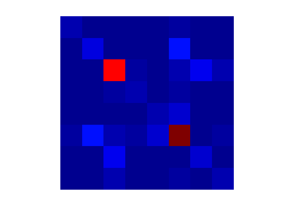
As we predicted from the raw aliased images, there is some increased noise in some channels.

Let's decoorelate:

dmtx = inv(chol(Rn,'lower'))*sqrt(2); %sqrt(2) for sd=1 in real and imag

%Both data and noise coil sensitivities
data_prew = ismrm_apply_noise_decorrelation_mtx(data,dmtx);
smaps_prew = ismrm_apply_noise_decorrelation_mtx(smaps,dmtx);

%Now let's repeat the reconstruction:
unmix_prew = ismrm_calculate_sense_unmixing(acc_factor,smaps_prew);

alias_img_prew = ismrm_transform_kspace_to_image(data_prew .* repmat(smask,[1 1 ncoils]),[1,2]);

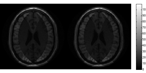
img_prew = sum(unmix_prew .* alias_img_prew,3);
ismrm_imshow(cat(3,abs(img),abs(img_prew)));

SNR Scaled Reconstruction

Now that we have performed noise-prewhitening, i.e. noise is scaled to sd=1, we would like to produce an image in SNR units.

For SNR scaled reconstruction, we need to make sure that all signal processing steps maintain SNR scaling.

Let's start by examining the transformation from k-space to image space:

%Generate white noise (like we have after prewhitening)
noise_white = complex(randn(size(data)),randn(size(data)));

%Mask out values that we don't acquire
noise_white = noise_white.*repmat(smask,[1 1 ncoils]);

%Transform from k-space to image:
noise_test = ismrm_transform_kspace_to_image(noise_white,[1,2]);

Get the standard deviation

sd = std(real(noise_test(:)))

sd =

    0.4986

As we can see the noise level is now about half of what it is supposed to be. This is because we have forgotten that only a quater of the samples are actually sampled and so we need to scale by the square root of the acceleration factor:

%Transform from k-space to image:
noise_test = sqrt(acc_factor)*ismrm_transform_kspace_to_image(noise_white,[1,2]);

%Now the standard deviation
sd = std(real(noise_test(:)))

sd =

    0.9972

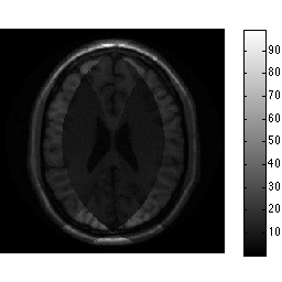
By scaling by the acceleration factor we have maintained unit noise scaling through our reconstruction. Now we can "trivially" obtain an SNR scaled reconstruction:

unmix_prew = ismrm_calculate_sense_unmixing(acc_factor,smaps_prew);

alias_img_prew = sqrt(acc_factor).*ismrm_transform_kspace_to_image(data_prew .* repmat(smask,[1 1 ncoils]),[1,2]);
img_snr = sum(unmix_prew .* alias_img_prew,3) ./ sqrt(sum(abs(unmix_prew).^2,3));

ismrm_imshow(abs(img_snr)); colorbar;

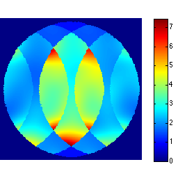
We can also easily inspect the g-map directly

gmap = sqrt(sum(abs(unmix_prew).^2,3)).*sqrt(sum(abs(smaps_prew).^2,3));
ismrm_imshow(abs(gmap)); colormap(jet); colorbar;

Pseudo Replica Method

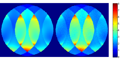
What if we didn't have access to the unmixing coefficients directly? We can obtain SNR scaled reconstructions using the pseudo replica method.

for r=1:100,
    noise_white = complex(randn(size(data)),randn(size(data)));
    noise_white = noise_white.*repmat(smask,[1 1 ncoils]);
    s = data_prew + noise_white;
    tmp = sqrt(acc_factor).*ismrm_transform_kspace_to_image(s .* repmat(smask,[1 1 ncoils]),[1,2]);
    img_noise_rep(:,:,r) = sum(tmp .* unmix_prew,3);
end

g_pseudo = std(abs(img_noise_rep + max(abs(img_noise_rep(:)))),[],3);
g_pseudo(g_pseudo < eps) = 1;
snr_pseudo = mean(img_noise_rep,3)./g_pseudo;
g_pseudo = g_pseudo.*sqrt(sum(abs(smaps_prew).^2,3));
ismrm_imshow([abs(img_snr) abs(snr_pseudo)]); colorbar;
ismrm_imshow([abs(gmap) abs(g_pseudo)]); colormap(jet); colorbar;

Iterative Non-Cartesian SENSE

Now let's look at non-Cartesian imaging. A spiral dataset is included in the example dataset.

First we noise pre-whiten

dmtx = ismrm_calculate_noise_decorrelation_mtx(noise_spiral);
data_spiral = ismrm_apply_noise_decorrelation_mtx(data_spiral,dmtx);
smaps_prew = ismrm_apply_noise_decorrelation_mtx(smaps,dmtx);

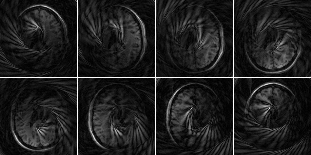
Then let us inspect the undersampled data

%Prepare NUFFT
N = [size(smaps,1) size(smaps,2)];
J = [5 5];
K = N*2;

nufft_st = nufft_init(k_spiral*2*pi,N,J,K,N/2,'minmax:kb');
recon_undersampled = nufft_adj(data_spiral .* repmat(w_spiral,[1 size(data_spiral,2)]),nufft_st);
ismrm_imshow(abs(recon_undersampled),[],[2 4]);

Low let's set up the non-Cartesian reconstruction First we need an encoding function to feed into LSQR:

dbtype ismrm_encoding_non_cartesian_SENSE.m

1     function outp =  ismrm_encoding_non_cartesian_SENSE(inp,csm,nufft_st,weights,transpose_indicator)
2     
3     scale = sqrt(prod(prod(nufft_st.Kd))/numel(weights(:)));
4     if (strcmp(transpose_indicator,'transp')),
5         samples = size(nufft_st.om,1);
6         coils = numel(inp)/samples;
7         inp = reshape(inp,samples,coils);
8         outp = (nufft_adj(inp .* repmat(sqrt(weights),[1 coils]),nufft_st)./(sqrt(prod(nufft_st.Kd))))*scale;
9         outp = sum(conj(csm) .* outp,3);
10        outp = outp(:);
11    elseif (strcmp(transpose_indicator, 'notransp')),
12        outp = repmat(reshape(inp,size(csm,1),size(csm,2)),[1 1 size(csm,3)]) .* csm;
13        outp = (nufft(outp,nufft_st)./(sqrt(prod(nufft_st.Kd))))*scale;
14        outp = outp .*repmat(sqrt(weights),[1 size(outp,2)]);
15        outp = outp(:);
16    else
17        error('Transpose flag not appropriately defined');
18    end
19    
20    return
21

Now let's set up the LSQR solver using this function

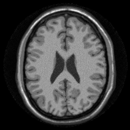
w = w_spiral*prod(K);
E = @(x,tr) ismrm_encoding_non_cartesian_SENSE(x,smaps_prew,nufft_st,w,tr);

img_spiral = lsqr(E, data_spiral(:) .* repmat(sqrt(w),[size(smaps_prew,3),1]),1e-3,50);
img_spiral = reshape(img_spiral,size(smaps_prew,1),size(smaps_prew,2));

ismrm_imshow(abs(img_spiral));

lsqr converged at iteration 47 to a solution with relative residual 0.059.

This functionality is encapsulated in the ismrm_non_cartesian_sense.m function.

help ismrm_non_cartesian_sense

    [img,snr,g,noise_psf] = ismrm_non_cartesian_sense(inp,k,w,csm,replicas)
 
    Non-Cartesian SENSE reconstruction. Uses Matlab LSQR to solve.
 
    It is recommended to input data with pre-whitened noise scale to sd=1.
 
    Gridding weights should be scaled such that sum(w(:)) is equal to the
    fraction of k-space that the samples cover, i.e. pi*0.5^2 for a circle.
 
    INPUT:
      - inp         [nsamples,coils]     : Input k-space data (vector)
      - k           [nsamples,2]         : k-space coordinates, range-0.5:0.5
      - w           [nsamples]           : vector of gridding weights
      - csm         [x,y,coil]           : Coil sensitivities 
      - reg         [x,y]                : Image space regularization mask
      - lambda      scalar               : regularization factor
      - replicas    scalar (dafault 100) : Number of replicas to run if SNR
                                           is requested
 
    OUTPUT:
      - img         [x,y]                : Output image
      - snr                              : An image in SNR units.
     -  g                                : A g-map (assuming image_formation_func doesn't scale)
     -  noise_psf                        : Point spread function of the noise
 
 
    Code made available for the ISMRM 2013 Sunrise Educational Course
  
    Michael S. Hansen (michael.hansen@nih.gov)

To reconstruct using this function use:

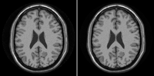
img_spiral2 = ismrm_non_cartesian_sense(data_spiral(:),k_spiral,w_spiral,smaps_prew);

ismrm_imshow(cat(3,abs(img_spiral),abs(img_spiral2)));

Warning: spdiag is superceded by diag_sp 
lsqr stopped at iteration 20 without converging to the desired tolerance 0.001
because the maximum number of iterations was reached.
The iterate returned (number 20) has relative residual 0.059.

For a demo on regularized non-Cartesian parallel imaging look in ismrm_demo_regularization_iterative_sense.m

Additional Demos

ismrm_demo_cartesian_snr_units.m

Reconstruction in SNR units using Cartesian data

ismrm_demo_iterative_cartesian.m

Cartesian iterative reconstruction. Demonstrates both SENSE and SPIRiT reconstruction techniques

ismrm_demo_noise_decorrelation.m

Demonstration of the effects of noise decorrelation.

*ismrm_demo_regularization_iterative_sense.m

Demonstration of the effects of regularization in non-Cartesian parallel imaging

ismrm_demo_non_cartesian.m

Demonstration of non-Cartesian parallel imaging with SENSE and SPIRiT