ISMRM Sunrise Practical Session, Parallel Imaging Part I

This document contains the first set of practical exercises for the ISMRM course on parallel imaging.

Exercise Data
Data Simulation
Prewhiten
Channel Combination
Create Acclerated Data
Create Data Driven & Model Driven Joint Encoding Relations
Use Various Calibration Approaches to Create Unmixing Images
Apply and Analyze Reconstructions
Additional Demos

Exercise Data

Exercise ground truth information is found in im1.mat (brain image), smaps_phantom.mat (sensitivity maps) and noise_covariances.mat (noise covariance matrices).

We start by clearing the workspace, loading this ground truth information and setting a few parameters from this.

close all;
clear all


fprintf('Loading Ground Truth Information\n');
load im1.mat
load smaps_phantom.mat
load noise_covariances.mat

ncoils = size(smaps,3);
Rn = Rn_normal_8;
imsize = size(im1);
nx = imsize(1);
ny = imsize(2);

Loading Ground Truth Information

Data Simulation

Let's use our ground truth data to simulate some data

channel_im = smaps .* repmat(im1, [1 1 ncoils]);

noise_scale = 0.1;
noise = noise_scale * max(im1(:)) * ismrm_generate_correlated_noise(imsize, Rn);
data = ismrm_transform_image_to_kspace(channel_im, [1 2]) + noise;

Prewhiten

Let's start by prewhitening so that we don't have to contend with the noise covariance matrix.

dmtx = ismrm_calculate_noise_decorrelation_mtx_from_covariance_mtx(Rn);
csm_true = ismrm_apply_noise_decorrelation_mtx(smaps, dmtx);
data = ismrm_apply_noise_decorrelation_mtx(data, dmtx);
%Rn = eye(ncoils);

Channel Combination

Let's use our ground truth data to perform an SNR-optimal channel combination

im_full = ismrm_transform_kspace_to_image(data, [1, 2]);
ccm_roemer_optimal = ismrm_compute_ccm(csm_true, eye(ncoils));
im_roemer_optimal = abs(sum(im_full .* ccm_roemer_optimal, 3));
ismrm_imshow(im_roemer_optimal);

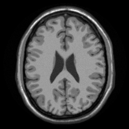
How does this compare to our ground-truth image?

ismrm_imshow(abs(im_roemer_optimal-im1));

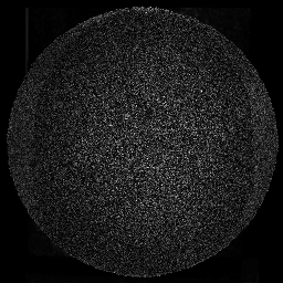
The noise level varies slightly from pixel-to-pixel. Let's make a map of this

noise_map = ismrm_calculate_noise_amplification(ccm_roemer_optimal, eye(ncoils));
ismrm_imshow(noise_map, [0 max(noise_map(:))]);

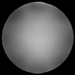
How does this compare to a root-sum-of-squares (SOS) reconstruction?

im_sos = ismrm_rss(im_full,3);
ismrm_imshow(cat(3, im_roemer_optimal, im_sos));
ismrm_imshow(cat(3, abs(im_roemer_optimal-im1), abs(im_sos-im1)));

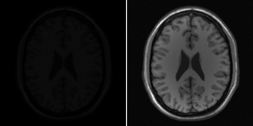
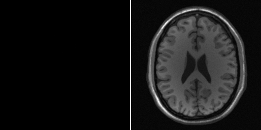
Looks like we have a scaling and/or shading issue that makes it hard to do this comparison. Let's normalize to SOS shading

[ccm_roemer_optimal, shading_correction_im] = ismrm_normalize_shading_to_sos(ccm_roemer_optimal);
im_roemer_optimal = abs(sum(im_full .* ccm_roemer_optimal, 3));
im_true = shading_correction_im .* im1;
ismrm_imshow(cat(3, im_true, im_roemer_optimal, im_sos));
ismrm_imshow(cat(3, abs(im_roemer_optimal-im_true), abs(im_sos-im_true)));

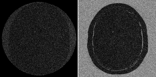
SOS channel combination aligns the phase of the background noise before summing, leading to a DC ofset in these pixels. Let's try channel combination based on coil sensitivity estimates from some low resolution calibration data.

cal_shape = [32 32];
cal_noise_scale = 0.1;
cal_data = ismrm_transform_image_to_kspace(channel_im, [1 2], cal_shape);
noise = cal_noise_scale * max(im1(:)) * ismrm_generate_correlated_noise(cal_shape, Rn);
cal_data = cal_data + noise;

cal_data = ismrm_apply_noise_decorrelation_mtx(cal_data, dmtx);

f = hamming(cal_shape(1)) * hamming(cal_shape(2))';
fmask = repmat(f, [1 1 ncoils]);
filtered_cal_data = cal_data .* fmask;

cal_im = ismrm_transform_kspace_to_image(filtered_cal_data, [1 2], imsize);

%
% Use a circular region of support for pixels
%
pixel_mask = sum(abs(smaps),3) > 0;
cal_im = cal_im .* repmat(pixel_mask, [1 1 ncoils]);

csm_walsh = ismrm_estimate_csm_walsh(cal_im);
csm_mckenzie = ismrm_estimate_csm_mckenzie(cal_im);

csm_true = ismrm_normalize_shading_to_sos(csm_true);
csm_walsh = ismrm_normalize_shading_to_sos(csm_walsh);
csm_mckenzie = ismrm_normalize_shading_to_sos(csm_mckenzie);

ccm_mckenzie = ismrm_compute_ccm(csm_mckenzie);
ccm_walsh = ismrm_compute_ccm(csm_walsh);

im_mckenzie = abs(sum(im_full .* ccm_mckenzie, 3));
im_walsh = abs(sum(im_full .* ccm_walsh, 3));

ismrm_imshow(cat(3, im_true, im_roemer_optimal, im_sos, im_walsh, im_mckenzie), [], [], {'source image', 'true csm', 'SoS', 'Walsh csm', 'McKenzie csm'});
ismrm_imshow(cat(3, abs(im_roemer_optimal-im_true), abs(im_sos-im_true), abs(im_walsh-im_true), abs(im_mckenzie-im_true)));

Create Acclerated Data

acc_factor = 4;
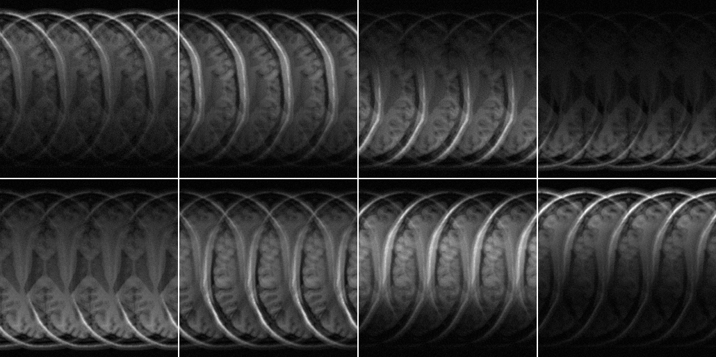
sp = ismrm_generate_sampling_pattern(imsize, acc_factor, 0);
data_accel = data .* repmat(sp == 1 | sp == 3,[1 1 ncoils]);
im_alias = ismrm_transform_kspace_to_image(data_accel,[1,2]);
ismrm_imshow(abs(im_alias),[], [2 4]);

Create Data Driven & Model Driven Joint Encoding Relations

kernel_shape = [5 7];
jer_lookup_dd = ismrm_compute_jer_data_driven(cal_data, kernel_shape);
unfiltered_cal_im = ismrm_transform_kspace_to_image(cal_data, [1,2], 2 * size(cal_data));
jer_lookup_md = ismrm_compute_jer_model_driven(unfiltered_cal_im, kernel_shape);

Use Various Calibration Approaches to Create Unmixing Images

num_recons = 4;
titles = {'SENSE true csm', 'SENSE estimated csm', 'PARS', 'GRAPPA'};

unmix = zeros([imsize ncoils num_recons]);
unmix(:,:,:,1) = ismrm_calculate_sense_unmixing(acc_factor, csm_true, eye(ncoils), 0) .* acc_factor;
unmix(:,:,:,2) = ismrm_calculate_sense_unmixing(acc_factor, csm_mckenzie, eye(ncoils), 0) .* acc_factor;
unmix(:,:,:,3) = ismrm_calculate_jer_unmixing(jer_lookup_md, acc_factor, ccm_mckenzie, 0, false);
unmix(:,:,:,4) = ismrm_calculate_jer_unmixing(jer_lookup_dd, acc_factor, ccm_mckenzie, 0, false);

SENSE unmixing

ismrm_imshow(abs(unmix(:,:,:,1)), [], [2 4]);
ismrm_imshow(angle(unmix(:,:,:,1)), [], [2 4]); colormap('hsv');

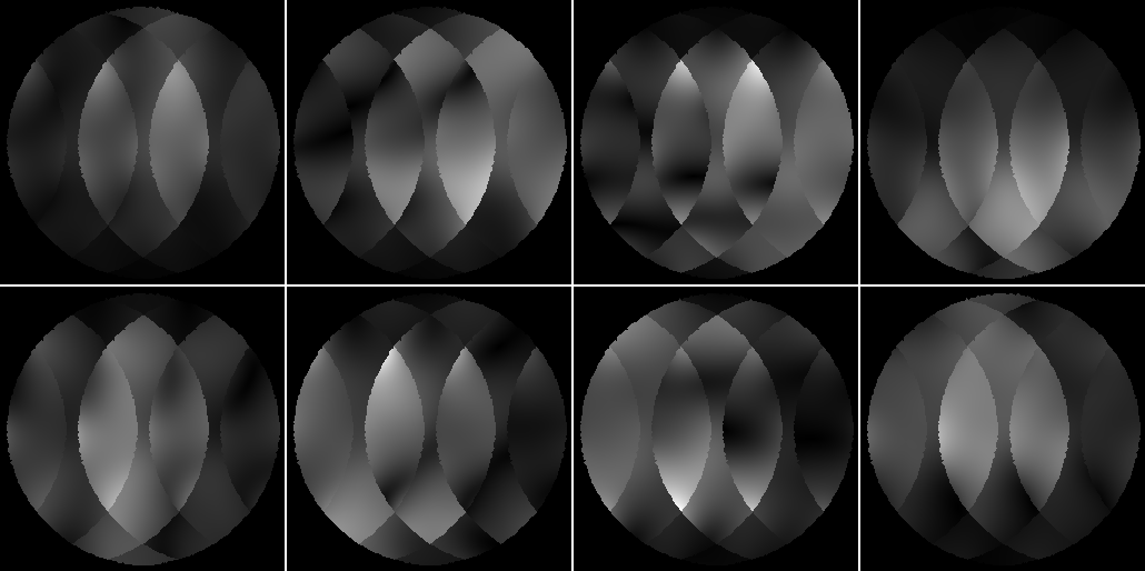
SENSE unmixing with estimated coil sensitivity maps

ismrm_imshow(abs(unmix(:,:,:,2)), [], [2 4]);
ismrm_imshow(angle(unmix(:,:,:,1)), [], [2 4]); colormap('hsv');

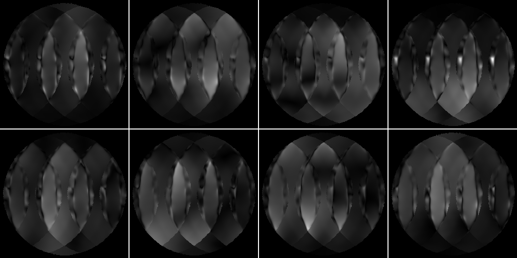
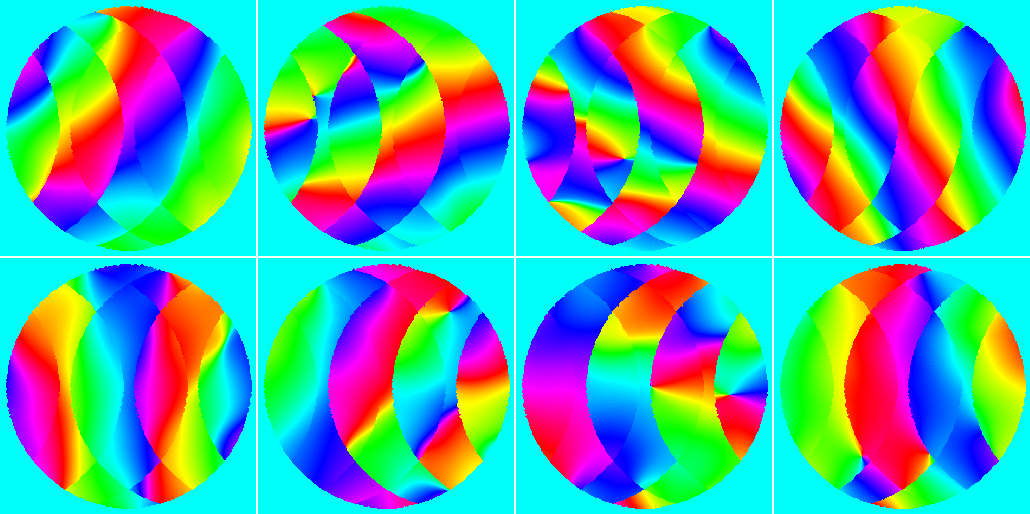
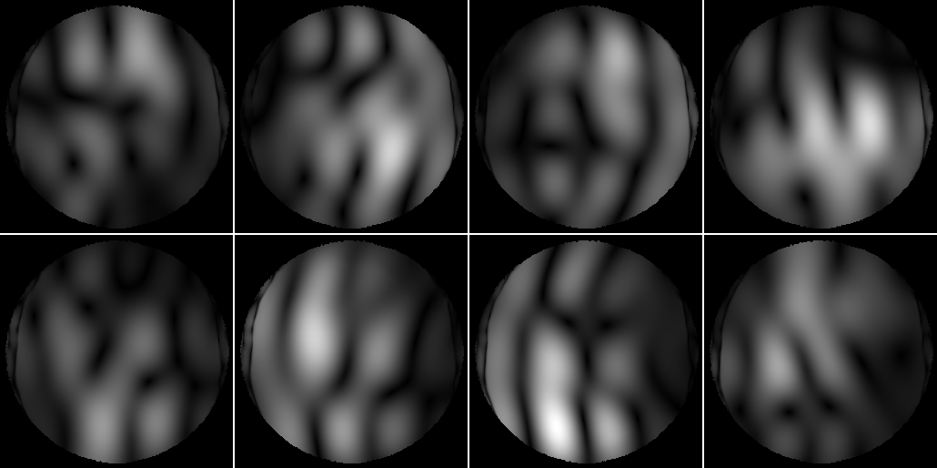
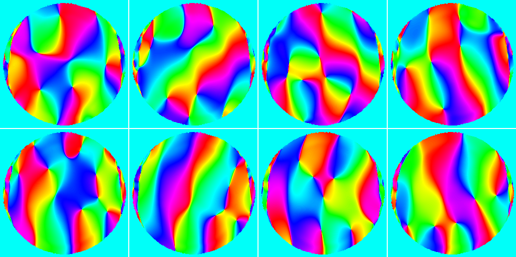
PARS unmixing

ismrm_imshow(abs(unmix(:,:,:,3)), [], [2 4]);
ismrm_imshow(angle(unmix(:,:,:,3)), [], [2 4]); colormap('hsv');

GRAPPA unmixing

ismrm_imshow(abs(unmix(:,:,:,4)), [], [2 4]);
ismrm_imshow(angle(unmix(:,:,:,4)), [], [2 4]); colormap('hsv');

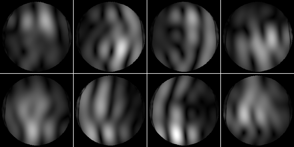
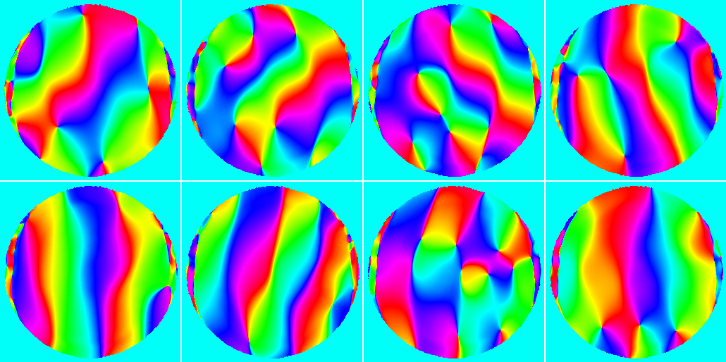
Apply and Analyze Reconstructions

aem = zeros([imsize num_recons]);
gmap = zeros([imsize, num_recons]);
im_hat = zeros([imsize, num_recons]);
im_diff = zeros([imsize, num_recons]);

signal_mask = imclose(im1>100.0, strel('disk', 5));

for recon_index = 1:num_recons,
    aem(:,:,recon_index) = ismrm_calculate_aem(signal_mask, csm_true, unmix(:,:,:,recon_index), acc_factor);
    gmap(:,:,recon_index) = ismrm_calculate_gmap(unmix(:,:,:,recon_index), ccm_roemer_optimal, Rn, acc_factor);
    im_hat(:,:,recon_index) = abs(sum(im_alias .* unmix(:,:,:,recon_index), 3));
    im_diff(:,:,recon_index) = abs(im_hat(:,:,recon_index) - im_true);
end

aliasing energy maps

ismrm_imshow(aem, [0 0.1], [], titles); colormap(jet);

g-factor (relative noise amplification) maps

ismrm_imshow(gmap, [0 6], [], titles); colormap(jet);

reconstructed images

ismrm_imshow(im_hat, [0 0.7 .* max(im_hat(:))], [], titles);

difference images

ismrm_imshow(im_diff, [0 0.1 * max(im_hat(:))], [], titles);

Additional Demos

ismrm_demo_prewhitening.m

Demonstration that prewhitening produces same end result as using the noise covariance matrix in the reconstruction.

ismrm_demo_rFOV.m

A study of the reduced field-of-view case.

ismrm_demo_minimal_cal.m

A study of calibration performance with a small number of calibration lines.

ismrm_demo_tychonov_regularization.m

A study of Tychonov regularization for SENSE and local k-space kernel calibration.